1 Basics

1.1 Create a new project

Create a new project with the name introduction-to-r
- Open RStudio by clicking on the icon or by selecting it via the start menu
- Click on File - New Project... and select New directory
- Give the directory the name introduction-to-r and create it as a sub-directory of your Desktop folder
- Where on your hard disk is the project folder located? Try to locate it with the regular windows file explorer.
Create a sub-directory data and source in the project’s root folder.
Download the titanic and the football dataset from the course website and place it in the data folder.
In RStudio type getwd() into the console window. This prints out the full path of your projects root folder.
- Type list.files("./data") into the console window. What’s the meaning of the dot . in the file path?
- What’s the output of the call list.files("../")?

1.2 Create a new script file (`helloWorld.R`)

Click on File - New File - R Script or use the plus button in the toolbar.
Write plot(rnorm(100)) into the text-editor
Execute the selected line by pressing [Strg]-[Enter] or by clicking on the Run button in the toolbar.
What’s the purpose of this command? Call the help page for the function rnorm.
Advanced: Write a small program which calculates the empricial mean and standard deviation for \(n=10\) random draws from the standard normal distribution.
- Use the functions mean, sd and rnorm
- E.g. type ?mean in the console to call the help page for this function
- What happens to the mean and deviation if \(n \rightarrow \infty\)? Try this in your program!
Save the file (File - Save) in the source folder of your project. Give it the name helloWorld.R.

1.3 KVB bikes in cologne

Download the script kvb.R from the course website and save it in the project’s source folder.
Install the missing packages XML and leaflet with the function install.packages
```
install.packages(c("XML", "leaflet"))
```
In your project in RStudio, open the script file and run the code line by line. Does the script terminate without any errors?
Advanced
- Change the color of the markers from red to green.
- Try to get and visualize data for another city in which nextbike operates (Inside the code, you have to change the link to the nextbike api).
- Add a cluster effect to the map (Use the function parameter clusterOptions = markerClusterOptions() at the right place).
- Change the pop-up text of the markers to display some other useful information such as the number of bikes at this place.

1.4 Arithmetic

Perform the following calcuations using the R console:

\(34^2 + 12^{-0.8}\)
\(\ln(4 + \sqrt{12})\)
\(\frac{2+1}{3+\pi}\)
\(\ln(e^4)\)

Advanced: \(\sqrt{2}^2 - 2 = 0\), right?

In R, why is sqrt(2)^2 - 2 not exactly equal to zero?
Do you find other examples?

1.5 Function calls

Have a look at the documentation for the function rnorm.
- How many arguments has the function?
- What are the default arguments of the function?
- Which of the following function calls is not valid? Why?
```
  rnorm(n = 10)
  rnorm(10, 2, 4)
  rnorm(mean = 2)
  rnorm(sd = 3, mean = 1, n = 3)
```
- With the help of the above function calls, explain how R matches formal to actual arguments!

2 Vectors and Operators

2.1 Basic data types

What are the three basic data types? Write down a code example for each of them.
What’s the difference between TRUE and "TRUE"? Whats the difference between pi and "pi"?
Use the function as.numeric() to cast values to a numeric type:
- What’s the numeric value of TRUE and FALSE?
- Can you cast the character string "hi" to a numeric value? Try the same with the string "5".
- How can you cast a numeric value to a string? To a logical value?

2.2 Vectors and variable assignment

Asign the value \(12\) to a variable with the name pi
- Why is this dangerous?
- Remove the variable by calling the rm() function with the appropriate argument.
Use the c() function to store the results from the calculations in exercise 1.4 in a vector . Assign the vector to a variable with the name values.
Try to find the name of the built-in functions and answer the following questions:
- What’s the sum and the product of the elements in the vector?
- What is the smallest/ largest value?
- How can you sort the vecor?
- How can you determine the length of the vector?
Call the ls() function to list all user variables in the global envrionment.
- How many variables are listed? Try to answer this question programmatically.
- What is the data type of the object returned by a call of ls()?

2.3 `descriptive.R`

Open a new script file and save it in the source folder under the name descriptive.R
Write a program which calculates the mean, the standard deviation, the range, the maximum and the minimum of an arbitrary numeric vector x
- You program should start with the following lines of code:
```
# define some arbitrary numeric vector with varying length e.g.
x <- c(1, 4, 2, 9)
# calculate the statistics
```
- Use only the built-in functions max(), min(), length() and sum()
- The range is defined as \(x_{max} - x_{min}\)

2.4 Vector generation

Try to generate the following sequences with the help of the functions c(), rep() and seq():
- \((1, 2, \dots, 100)\)
- \((-10, -9.5, -9, -8.5, \dots, -4.5, -4)\)
- \((TRUE, FALSE, TRUE, FALSE, TRUE, FALSE)\)
- \(("A", "B", "C", "A", "B", "C", "A", "B", "C")\)
- \((100, 90, 80, \cdots, 10, 0, -10)\)
Advanced (Tip: Have a look at the documentation for the function rep()):
- \((1, 1, 1, 2, 2, 2, 3, 3, 3, 4, 4, 4, \cdots, 100, 100, 100)\)
- \((1, \dots, 100, 1, \dots, 100, 1, \dots, 100, 1, \dots, 100)\)
- \((1000000, 100000, 10000, 1000, 100, 10, 1)\)

2.5 Casting

Have a look at the two vectors:

x <- c("TRUE", "FALSE", "TRUE", "TRUE")
y <- c("2", "4", "5")

Execute the following expressions in R and explain the result.

as.numeric(as.logical(x))
is.numeric(y)
is.character(x)
is.logical(as.character(TRUE))

Try to guess the result of the following expressions without using a computer

is.logical(0)
is.logical(as.logical(0))
is.numeric(as.logical(x))
as.character(1243)

2.6 Logical expressions

Have a look at the two values x and y and the vector a and b

x <- 9^2
y <- "test"
a <- c(4, 6, 5, 7, 10, 9)
b <- c(4, 6, 2, 7, 2, 3)

Execute the following expressions in R and try to explain the result

(4 < 5) & (sqrt(x) == 9)
y == "Test" | y == "test"
x < 100 | y != "hallo"

a > 5 & b < 7
all(a > 4 | b < 6)
any(a < 2)
length(a) == length(b)

Try to guess the result of the following expressions without using a computer

a < 4 & b > a
a == length(b)
any(sqrt(x) == a)
all(a < b)
length(x)

2.7 Logical expressions and vectorization

Create a vector of logical values and apply the sum() and mean() function to it. What do you observe?
With the function rnorm(), sample \(n = 100\) values from the normal distribution. Count the relative and absolute number of observations which are
- positive
- between \(-1\) and \(1\)
- larger than two times the empirical standard deviation of the sample
Advanced: Given the previous three expressions, calculate the analytical probability values with the function pnorm() for some random normal variable with \(X \sim N(\mu_x,\sigma_x)\). E.g. calculate the probabilities:
- \(P(X > 0)\)
- \(P(-1 \leq X \leq 1)\)
- \(P(X > 2\sigma_x)\)

2.8 Missing values

What is the keyword for a missing value? Create a vector with numeric values and some missing values.
Use the function is.na() on your vector to test for missing values. What is the return type of the function is.na()?
Use the sum() function together with is.na() to count the number of missing values in the vector.
Have a look at your code in descriptive.R.
- What happens to the code, if the vector x contains missing values?
- Try to rewrite your code such that missing values are handled (E.g. look at the further function arguments of the functions mean(), sum(), …).
- Expand the code by an expression, which counts the number of missing values.

3 Data import and data frames

3.1 `.csv` data

Open the titanic dataset with a text editor (e.g. right click on the file - edit with notepad++)

How many variables/columns has the dataset?
How many passengers are included in the dataset?
Does the file contain a header line?
How are the values separated?
What’s the encoding of the file?

3.2 The titanic dataset

Open a new script file, save it in source and give it the name titanic.R.
Use the read.csv() function with the correct file path, to import the titanic dataset into R (Remember to also include the argument stringsAsFactors = FALSE).
Have a look at each column and determine it’s datatype. You can also use the summary() or the head() function for this.
Try to answer the following questions programmatically:
- How many passengers and which variables are included in the dataset?
- How many people died on the titanic? How many people survived? Calculate the overal survival rate (E.g. the number of survivors as a fraction of the overall number of passengers).
- How many of the passengers are women?
- How many missing values does the variable age contain?
- What’s the age of the youngest and oldest passenger on the titanic?
- How many passengers are in the first class?

3.3 Frequency tables

With the titanic dataset and the function table() answer the following questions:

How many men are in the third class?
How many people died in the first class? How many in the third class?

In addition, use the functions prop.table() to transform the tables into relative frequency tables:

Calculate the survival rate separately for each class. Did people from the first class had a higher chance to survive?
Did women have a higher chance to survive?

3.4 Variable creation and updating

Add a new column isMale to the dataset which is TRUE if the passenger is male.
Change the data-type of the survived column from numeric to logical.
Add a new column isChild to the dataset which is TRUE if age < 18 and FALSE else. Are missing values preserved?
Advanced: Add a new column which is TRUE if the name contains the string "Miss" and FALSE else.
- Use the function grepl()
- Did unmarried woman had a greater chance to survive?

3.5 Advanced: Significant differences in the survival rates (chi sqared test)

Use the function chisq.test to check if there is a significant relationship between the class and the survival rate of a personen.

Use the table function to create a contingency table.
Whats the null hypothesis of the test?
How large is the p-value and what can you conclude?

3.6 Advanced: The football dataset

Import the football dataset using the read.csv2() function. Why do you have to use read.csv2() instead of read.csv()?
How many games are in the dataset?
How many unique countries are included in the dataset?
How many games from the FIFA World Cup are included in the dataset?
Think of some questions you want to answer with the dataset and if you can allready answer them with the tools you have learned so far.

4 Functions and control structures

4.1 Function `countMissings()`

Write a function countMissings which accepts a numeric vector x as input argument and returns the number of missing values NA in the vector.

Use this template as a start:

countMissings <- function(x){
  # calculate nMissings here

  # return the number of missing values
  return(nMissings) 
}

Apply the function to the age variable from the titanic dataset.
Advanced: If the vector contains only missing values, a warning should be printed to the console. Use the function warning() and an if construct for this.

4.2 Turn `descriptive.R` into a function

Wrap your code from descriptive.R into a function with the name descriptive(). The function accepts a numeric vector x as input argument, calculates the descriptive statistics and returns them in a named vector. Use this template as a start:

descriptive <- function(x){
  # calculate the descriptive statistics for x here
  
  # return the result
  return(result) # result should be a named vector containing the descritpive statistics
}

Tip: You can create a named vector like this:
```
result <- c(mean = 0.4, sd = 4, range = 2)
```
Apply the function descriptive() to the survived and pclass column from the titanic dataset.
Advanced: What happens if you apply your function to the age variable which contains missing values. Think of ways to correctly handle missing values (e.g. you could add an additional argument removeNA to your function)
Advanced: If the type of the vector x is not numeric, the function should terminate with an error (look at the function stop()).

4.3 The `sapply()` function

use sapply() with the countMissings() function from exercise \(4.1\) to count the number of missing values in each column of the titanic dataset.

4.4 Visibility of variables

What’s wrong with the following lines of code? Rewrite the function mySum such that it can be used without errors.

mySum <- function(a){# calculates the sum of two numbers a and b
  return(a+b)
}
mySum(4)
b <- 6
mySum(2)

Look at the following code:

norm <- function(x){# calculates the eucledian norm of a vector
  xNorm <- sqrt(sum(x^2))
  return(xNorm)
}
x <- c(1, 2, 1)
x <- norm(x)
xNorm
x

Does the code terminate without any errors? Where is the mistake? Correct the mistake.
In this example, what’s the formal and the actucal argument of the function norm()?
What’s the value of the variable x after the code terminates?

4.5 Advanced: Function `normalize()`

Write a function normalize() which standardizes a numeric vector x such that \[ x_{norm} = \frac{x-\bar{x}}{x_{sd}} \]
- If the vector contains missing values a warning via the function warnings() should be printed to the console.
- If the vector is not numeric (e.g. it contains logical values), the function should be terminating with an error. Use the function stop() and is.numeric().
Rewrite the function normalize such that the user can pass two parameters mand s with \[ x_{norm} = \frac{x-m}{s} \]
- Think of downward compability: A user should still be able to call the function via normalize(x). You can achieve this by using default arguments.

5 Extraction and updating

5.1 Vector subsetting

Which methods for extracting values from a vector do you know?
Sample \(n = 100\) values from the standard normal distribution and subset the sample by selecting
- only positive values
- values between \(-1\) and \(1\)
- the first and the last value
- everything but the first value

5.2 Test

Look at the two vectors:

x <- c(2, 3, 4, 4)
y <- c(TRUE, FALSE, FALSE, TRUE)

Without using a computer: What’s the result of the following expressions?

sum(x[y])
sum(x[!y])
sum(y[x])
sum(y[-x])
# advanced
which(x > 3)
which(x[y] > 3)

5.3 Remove missing values from a vector

How can you remove missing values from a vector? Write a function removeNA() which takes some numeric vector x as input and returns the vector with missing values removed.

Find an expression for selecting only non-missing values from the vector x (e.g. use the function is.na together with extraction method [])
Inside the function create a variable xClean containing the subset of x with the missing values removed
Return the vector xClean

A call of this function should look like this:

x <- c(2, 3, NA, 4)
removeNA(x)

[1] 2 3 4

5.4 Set negative numbers to zero

Write a function negToZero() which sets negative numbers in a vector x to \(0\). A call of this function should look like this:

x <- c(-10, 3, -2, 3, 4)
negToZero(x)

[1] 0 3 0 3 4

5.5 Advanced: Recoding

Write a function codeToNA() which converts some user defined numbers in a vector x into NAs.

Tip: Use the %in% operator to update the values inside the vector x.
To understand how the %in% operator works, have a look at this example: 1:10 %in% c(1,3,5,9)

A call of this function looks like this:

x <- c(2, 3, -99, -999, NA, 4)
codeToNA(x, c(-99, -999))

[1]  2  3 NA NA NA  4

5.6 Outlier detection

Write a function removeOutliers() which identifies positive outliers in a numeric vector x.

Here, a positive outlier \(x_i\) is defined as \(x_i: x_i > \bar{x} + 3*sd(x)\).
The function should return the vector without outliers.
Advanced: Enhance the functionality by allowing the user to specify if only positive, only negative or both positive and negative outliers should be removed.

A call of this function looks like this:

x <- c(2, 3, 120,1.5, 2, 1, 0, 999)
removeOutliers(x)

[1]   2.0   3.0 120.0   1.5   2.0   1.0   0.0

Advanced: You can also write a function detectOutliers which gives the indices of the outliers in a vector. Are there any outliers in the age column of the titanic dataset?

5.7 Extraction and updating of data frames

Add a new column ageImputed to the dataset which contains the age of the passenger but with NAs replaced by the overall average age (see Mean imputation).
Create a copy of the titanic dataset for which the passengers (e.g. the rows) with a missing value are removed.
Filter the titanic dataset and select only:
- the survivors
- women in the first class
- male children.

5.8 Advanced: Two sample t-tests

What is the average age for passengers which have a Miss in their name (comare with exercise 3.4)?
Use the function t.test to perform a two sample t-test and check wether the difference in the mean age between Misses and all other passengers is significant.
What’s the meaning of the confidence interval?
Use the same test but now just use a one-sided test (e.g. test if the difference in the means is less than zero).

5.9 Ordering of data frames

Order the rows of the titanic dataset such that the age is in decreasing order.
What’s the name and age of the youngest/ the oldest passenger? Did he or she survive?
Advanced: Select the top \(10\) youngest passengers from each class. How many of them survived?

6 Visualizations

6.1 Step by step visualization

Complete the step by step visualization from the slides
Add additional elements or labels
Change the colors, the point size or the line type
Save your plot as a pdf document

6.2 Visualization examples

Choose a visualization from the examples on the slides and complete the plot, e.g.
- add a title, subtitle, caption
- change the theme
- …

6.3 Visualization project

Form groups of two to four and choose a dataset
Develope a small research question or replicate a question from the exercises
In a new .R script file read in the data, clean and transform it
If needed, apply a regression model or conduct a statistical test
Create 1 or 2 visualizations and upload the code to ILIAS
- Make sure that your script file contains no errors, is readable and sharable

7 Advanced exercises

7.1 Matrics

Use the matrix function and create the following matrics \[ A= \begin{pmatrix} 2 & 4 \\ 1 & 6 \\ \end{pmatrix} , B = \begin{pmatrix} 1 & 3 & 9\\ 8 & 2 & 4\\ \end{pmatrix} , C = \begin{pmatrix} TRUE & TRUE & FALSE\\ TRUE & FALSE & TRUE\\ \end{pmatrix} \] Calculate

\(A*B\)
\(B'*A\)
\((A*B*A')^{-1}\).

7.2 Two-sample t-test for equal means

Write a function myTTest which tests, if the mean of two given numeric vectors x and y is statistically different from one another (see here for a detailed explanation)
- The input arguments of the function are the vectors x, y and a significance level alpha
- The null hypothesis is: \(H_0: \mu_x = \mu_y\).
- The test value can be calculated as: \[ T = \frac{\bar{x}-\bar{y}}{\sqrt{\frac{1}{n}x_{sd}^2+ \frac{1}{m}y_{sd}^2}} \]
- \(H_0\) is rejected if \(|T| > u_{1-\frac{\alpha}{2}}\)
- \(n\), \(m\) are the length of the vectors \(x\) and \(y\)
- \(u_{1-\frac{\alpha}{2}}\) is the quartile of the normal distribution (see qnorm())
- The function should return a list with the mean of each of the two vectors, the test value and a logical value indicating the test result
Compare your results with the built in function t.test
Advanced
- Calculate p-values or produce a nice output (e.g. with stars indicating the strength of significance)
- If the sample size \(n,m<40\) a warning should be printed (see warning())

7.3 Write your own linear regression function

Write a function myRegression which performs a multivariate linear regression analysis given some outcome y and some design matrix X. The model is given by the equation: \[ y = X\beta + \epsilon,~ \epsilon \sim N(0, \sigma^2) \] The function should calculate the following statistics:

The regression coefficients: \(\hat{\beta} = (X'X)^{-1}X'y\)
The number of observations \(N\) and the number of regressors \(K\)
The residuals: \(e = y - X\hat{\beta}\)
The error variance \(\hat{\sigma^2} = \frac{\sum_{i = 1}^{N}{e_i^2}}{N-K}\)
The coefficient of determination \(R^2 = 1 - \frac{\sum_{i = 1}^{N}{e_i^2}}{\sum_{i = 1}^{N}{(y_i - \bar{y})^2}}\)

The results should be returned using a named list. Check your calculations using the built-in function lm.

Advanced: Enhance the function with a t-test for the coefficients and calculate p-values and confidence intervals

Tip: R can do matrix arithmetic such as addition, multiplication and inversion: Have a look at help("%*%") and ?solve

7.4 Modelling survival rates with linear regression

Use the titanic dataset and the examples from to slides:

Run a simple linear regression model with the formula survived ~ ageImputed. Is the age significant (ageImputed was calculated in exercise 5.7)?
In addition, include the pclass and the sex as independent variables. Is the age now significant?
In the model above, what’s the effect of the age on the survival rate (E.g. how much does the probability of survival decreases for passenger who is one year older)?
Include the embarked variable. Are there any significant effects?
Use the predict.lm function to predict the probability of survival for each passenger. Compare the predicitons to the real outcome. How good is the fit?
Advanced: What’s the probability of survival for a \(20\) year old male in the third class? Use the predict.lm() function with the newdata argument.

7.5 String operations

Try to squeeze out some information from the name column in the titanic dataset:

Look for family names and - together with the columns embarked and pclass - identify family members.
Extract the title (e.g. Mr, Miss, Master, …) from the name.
What else can you do?

Tip: Install the stringr package, load it with library(stringr) and have a look at the various functions having the naming convention: str_<action>() (e.g. str_replace(), str_detect()).

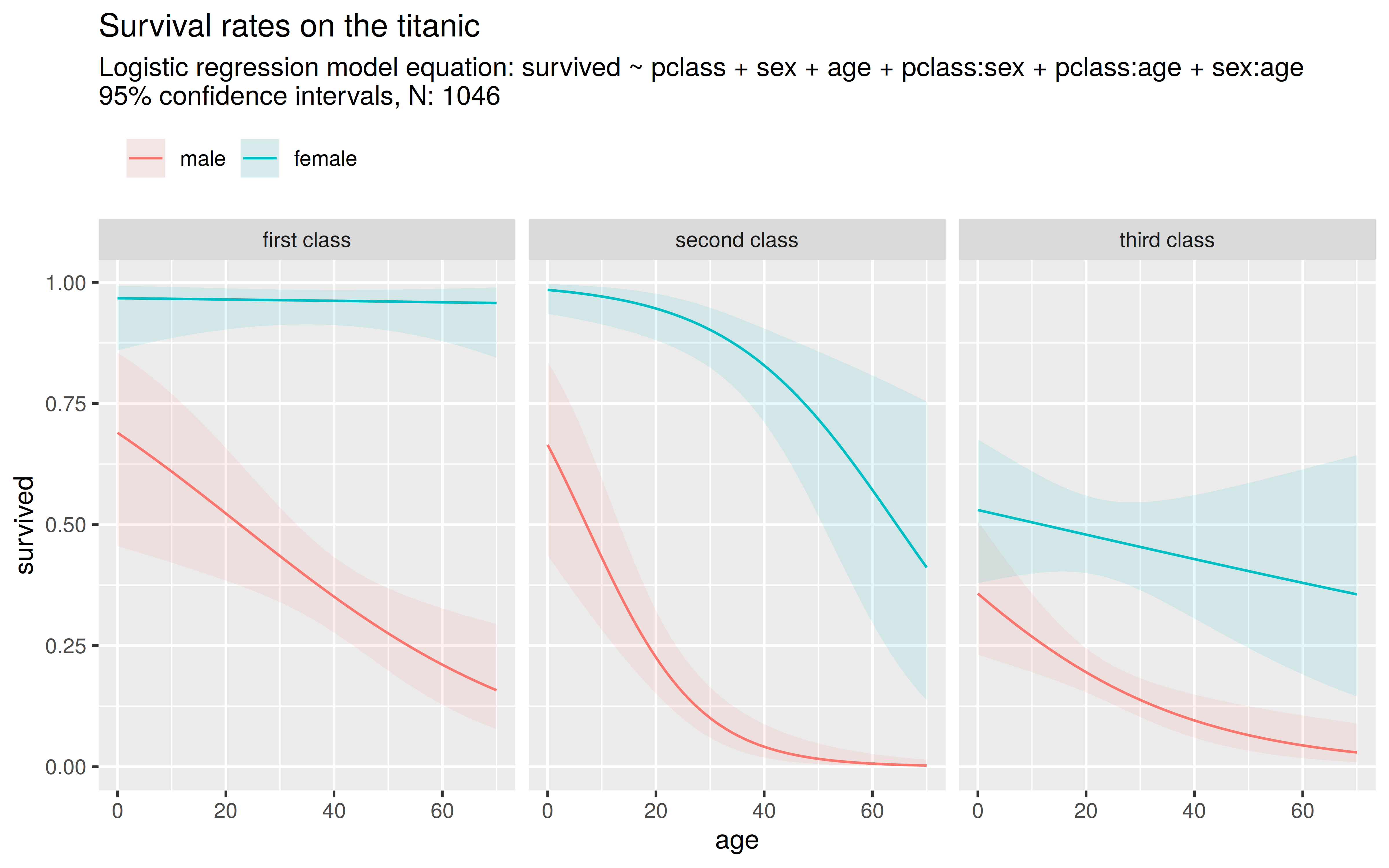
7.6 Logistic regression modelling and visualization

Use the ggplot2 package, the glm() function and the titanic dataset to model and visualize survival rates on the titanic. Use a logistic regression model with the independent variables age, pclass and sex and the dependent variable survived.

The final figure could look like this (A script to produce this figures can be found in the scripts section):

A guidance on how to proceed:

Import the titanic dataset and use the function as.factor() to transform the pclass and the sex variable into the factor datatype.
Use the glm function with the formula: survived ~ pclass + sex + age + pclass:sex + pclass:age + sex:age and the family = "binomial" argument.
- with the : in the formula, interaction effects can be specified
- with family = "binomial" one can specify a logistic regression model
Apply the summary() function to the model object and try to interpretate the coefficients. Why is it important to transform the pclass variable to the factor datatype befor applying the model?
Use the model, to predict survival rates over the possible range of age, sex and pclass
- with the expand.grid() function, create a new data.frame filled with “artifical” passenger data: for each possible outcome of sex and pclass you should vary the age from \(0-70\).
- It is important that the new data has the same columns names as the variable names in the model (e.g. sex, pclass and age).
- use the function predict() on the model object and the new data to predict the survival rates.
- add a new column with the predictions to the data.frame containing the new passenger data.
Use the ggplot() function to plot the passenger data
- Define the asthetics inside ggplot() with the aes() function. Use the asthetics x, y and color.
- Add the trend lines with geom_line()
- Use facet_grid(~pclass) to create three separate plots
- Add a title with ggtitle()
Further steps: Find out how to add confidence bars to the plot
- The predict() function can return standard errors for the predictions
- The geom_ribbon() function adds an interval arround the trend lines. Use the additional asthetics ymin for the lower confidence bound, ymax for the upper confidence bound and fill for the transparent fill color.

Introduction to R - Exercises